6. KMeans Clustering and Results
Written by Men Vuthy, 2021
Import packages
[1]:
import os
import rasterio
import rasterio.mask
import numpy as np
import pandas as pd
import seaborn as sns
import matplotlib.pyplot as plt

# sklearn & Scipy Libraries
from sklearn.cluster import KMeans
from sklearn.metrics import accuracy_score

import fiona
Input Feature Data
[2]:
# Reading dataset
NN_NDVI = pd.read_csv('output/3/no_noise_data/no_noise_ndvi.csv')

# Data manipulation
Input_DF = NN_NDVI.iloc[4:,:].T
Input_DF
[2]:
| 4 | 5 | 6 | 7 | 8 | 9 | 10 | 11 | 12 | 13 | ... | 59 | 60 | 61 | 62 | 63 | 64 | 65 | 66 | 67 | 68 | |
|---|---|---|---|---|---|---|---|---|---|---|---|---|---|---|---|---|---|---|---|---|---|
| 464 | 0.51950 | 0.57864 | 0.63714 | 0.64732 | 0.67500 | 0.67774 | 0.68980 | 0.69454 | 0.69234 | 0.67418 | ... | 0.66744 | 0.65592 | 0.61508 | 0.53592 | 0.49996 | 0.49064 | 0.52672 | 0.50306 | 0.58068 | 0.62020 |
| 465 | 0.53694 | 0.54528 | 0.59784 | 0.63970 | 0.65370 | 0.65422 | 0.68336 | 0.69858 | 0.65140 | 0.63988 | ... | 0.59776 | 0.47894 | 0.32178 | 0.20738 | 0.12034 | 0.03210 | 0.13908 | 0.17912 | 0.24692 | 0.30328 |
| 466 | 0.55552 | 0.58060 | 0.64768 | 0.68540 | 0.67414 | 0.67482 | 0.69040 | 0.69288 | 0.63874 | 0.59288 | ... | 0.59052 | 0.41846 | 0.25602 | 0.13288 | 0.04092 | -0.03880 | 0.11154 | 0.11886 | 0.20148 | 0.26276 |
| 467 | 0.55560 | 0.63836 | 0.66420 | 0.70210 | 0.69084 | 0.71550 | 0.72062 | 0.72310 | 0.68032 | 0.60178 | ... | 0.51830 | 0.37740 | 0.24368 | 0.16522 | 0.09862 | 0.03156 | 0.12450 | 0.13378 | 0.21640 | 0.29612 |
| 1215 | 0.70558 | 0.74582 | 0.74244 | 0.73444 | 0.75022 | 0.73344 | 0.73354 | 0.73058 | 0.73094 | 0.71617 | ... | 0.67193 | 0.62406 | 0.58591 | 0.49347 | 0.54397 | 0.51235 | 0.55181 | 0.59130 | 0.67986 | 0.69842 |
| ... | ... | ... | ... | ... | ... | ... | ... | ... | ... | ... | ... | ... | ... | ... | ... | ... | ... | ... | ... | ... | ... |
| 391324 | 0.80152 | 0.79928 | 0.79852 | 0.80118 | 0.79846 | 0.76344 | 0.76540 | 0.77446 | 0.76666 | 0.65752 | ... | 0.65426 | 0.57752 | 0.62126 | 0.56004 | 0.48050 | 0.53128 | 0.56300 | 0.50778 | 0.57666 | 0.69396 |
| 391325 | 0.82454 | 0.82177 | 0.82139 | 0.82083 | 0.76687 | 0.75187 | 0.74798 | 0.75704 | 0.72350 | 0.75358 | ... | 0.61884 | 0.61610 | 0.65594 | 0.61808 | 0.45692 | 0.53786 | 0.42998 | 0.28714 | 0.36382 | 0.53096 |
| 392074 | 0.83522 | 0.82322 | 0.82546 | 0.82742 | 0.82954 | 0.81118 | 0.73832 | 0.74184 | 0.70344 | 0.60238 | ... | 0.61174 | 0.61277 | 0.69493 | 0.66797 | 0.65902 | 0.75882 | 0.74525 | 0.74403 | 0.76445 | 0.77786 |
| 392075 | 0.83498 | 0.83440 | 0.83656 | 0.83886 | 0.84306 | 0.82860 | 0.74522 | 0.74880 | 0.72850 | 0.61764 | ... | 0.54754 | 0.46808 | 0.53508 | 0.50970 | 0.46386 | 0.57238 | 0.64828 | 0.58970 | 0.61062 | 0.73332 |
| 392076 | 0.80760 | 0.80264 | 0.80284 | 0.79794 | 0.79396 | 0.74928 | 0.75226 | 0.75998 | 0.71980 | 0.61102 | ... | 0.54766 | 0.49084 | 0.55458 | 0.57926 | 0.55106 | 0.59722 | 0.56852 | 0.47848 | 0.50222 | 0.62462 |
192289 rows × 65 columns
[3]:
# Set X as input feature data
X_KMeans = Input_DF
Elbow Method
Elbow curve method is used to identify the ideal number of clusters.
[4]:
# Let's use the elbow curve method to identify the ideal number of clusters
Error = []
for i in range(1, 11):
    kmeans = KMeans(n_clusters = i).fit(X_KMeans)
    kmeans.fit(X_KMeans)
    Error.append(kmeans.inertia_)
[5]:
plt.plot(range(1, 11), Error)
plt.title('Elbow method')
plt.xlabel('No of clusters')
plt.ylabel('Error')
plt.show()
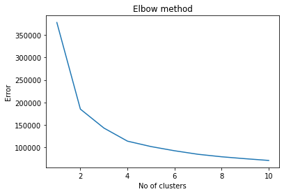
Based on the curve, 6 clusters are used.
Classification
[6]:
# Apply KMeans clustering
kmeans = KMeans(n_clusters=6, init='k-means++', max_iter=500, random_state=42)

Y_KMeans = kmeans.fit(X_KMeans)
[7]:
# Assign label
X_group = X_KMeans.copy()
X_group['cluster_id'] = kmeans.labels_
X_group.head()
[7]:
| 4 | 5 | 6 | 7 | 8 | 9 | 10 | 11 | 12 | 13 | ... | 60 | 61 | 62 | 63 | 64 | 65 | 66 | 67 | 68 | cluster_id | |
|---|---|---|---|---|---|---|---|---|---|---|---|---|---|---|---|---|---|---|---|---|---|
| 464 | 0.51950 | 0.57864 | 0.63714 | 0.64732 | 0.67500 | 0.67774 | 0.68980 | 0.69454 | 0.69234 | 0.67418 | ... | 0.65592 | 0.61508 | 0.53592 | 0.49996 | 0.49064 | 0.52672 | 0.50306 | 0.58068 | 0.62020 | 0 |
| 465 | 0.53694 | 0.54528 | 0.59784 | 0.63970 | 0.65370 | 0.65422 | 0.68336 | 0.69858 | 0.65140 | 0.63988 | ... | 0.47894 | 0.32178 | 0.20738 | 0.12034 | 0.03210 | 0.13908 | 0.17912 | 0.24692 | 0.30328 | 2 |
| 466 | 0.55552 | 0.58060 | 0.64768 | 0.68540 | 0.67414 | 0.67482 | 0.69040 | 0.69288 | 0.63874 | 0.59288 | ... | 0.41846 | 0.25602 | 0.13288 | 0.04092 | -0.03880 | 0.11154 | 0.11886 | 0.20148 | 0.26276 | 2 |
| 467 | 0.55560 | 0.63836 | 0.66420 | 0.70210 | 0.69084 | 0.71550 | 0.72062 | 0.72310 | 0.68032 | 0.60178 | ... | 0.37740 | 0.24368 | 0.16522 | 0.09862 | 0.03156 | 0.12450 | 0.13378 | 0.21640 | 0.29612 | 2 |
| 1215 | 0.70558 | 0.74582 | 0.74244 | 0.73444 | 0.75022 | 0.73344 | 0.73354 | 0.73058 | 0.73094 | 0.71617 | ... | 0.62406 | 0.58591 | 0.49347 | 0.54397 | 0.51235 | 0.55181 | 0.59130 | 0.67986 | 0.69842 | 1 |
5 rows × 66 columns
[8]:
# Checking how many data points are there in each cluster
X_group['cluster_id'].value_counts()
[8]:
5    51797
4    41958
2    30122
1    28829
0    25071
3    14512
Name: cluster_id, dtype: int64
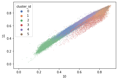
[9]:
# Scatter plot
sns.scatterplot(x=10, y = 11, hue = 'cluster_id', s=1, data = X_group, palette="deep");
Validation
[10]:
# Read validation data
DF_Validation = pd.read_csv('output/4/validation_data/validation_paddy.csv')

X_Validation = DF_Validation.T
[11]:
# Y true
Y_Validation = np.full((250,), 2, dtype='int32')
Y_Validation
[11]:
array([2, 2, 2, 2, 2, 2, 2, 2, 2, 2, 2, 2, 2, 2, 2, 2, 2, 2, 2, 2, 2, 2,
       2, 2, 2, 2, 2, 2, 2, 2, 2, 2, 2, 2, 2, 2, 2, 2, 2, 2, 2, 2, 2, 2,
       2, 2, 2, 2, 2, 2, 2, 2, 2, 2, 2, 2, 2, 2, 2, 2, 2, 2, 2, 2, 2, 2,
       2, 2, 2, 2, 2, 2, 2, 2, 2, 2, 2, 2, 2, 2, 2, 2, 2, 2, 2, 2, 2, 2,
       2, 2, 2, 2, 2, 2, 2, 2, 2, 2, 2, 2, 2, 2, 2, 2, 2, 2, 2, 2, 2, 2,
       2, 2, 2, 2, 2, 2, 2, 2, 2, 2, 2, 2, 2, 2, 2, 2, 2, 2, 2, 2, 2, 2,
       2, 2, 2, 2, 2, 2, 2, 2, 2, 2, 2, 2, 2, 2, 2, 2, 2, 2, 2, 2, 2, 2,
       2, 2, 2, 2, 2, 2, 2, 2, 2, 2, 2, 2, 2, 2, 2, 2, 2, 2, 2, 2, 2, 2,
       2, 2, 2, 2, 2, 2, 2, 2, 2, 2, 2, 2, 2, 2, 2, 2, 2, 2, 2, 2, 2, 2,
       2, 2, 2, 2, 2, 2, 2, 2, 2, 2, 2, 2, 2, 2, 2, 2, 2, 2, 2, 2, 2, 2,
       2, 2, 2, 2, 2, 2, 2, 2, 2, 2, 2, 2, 2, 2, 2, 2, 2, 2, 2, 2, 2, 2,
       2, 2, 2, 2, 2, 2, 2, 2])
[12]:
# Y prediction
Y_Prediction = kmeans.predict(X_Validation)
Y_Prediction
[12]:
array([2, 2, 2, 2, 2, 2, 2, 2, 2, 2, 2, 2, 2, 2, 2, 2, 2, 2, 2, 2, 2, 2,
       2, 2, 2, 2, 2, 2, 2, 2, 2, 2, 2, 2, 2, 2, 2, 2, 2, 2, 2, 2, 2, 2,
       2, 2, 2, 2, 2, 2, 2, 2, 2, 2, 2, 2, 2, 2, 2, 2, 2, 2, 2, 2, 2, 2,
       2, 2, 2, 2, 2, 2, 2, 2, 2, 2, 2, 2, 2, 2, 2, 2, 2, 2, 2, 2, 2, 2,
       2, 2, 2, 2, 2, 2, 2, 2, 2, 2, 2, 2, 2, 2, 2, 2, 2, 2, 2, 2, 2, 2,
       2, 2, 2, 2, 2, 2, 2, 2, 2, 2, 2, 2, 2, 2, 2, 2, 2, 2, 2, 2, 2, 2,
       2, 2, 2, 2, 2, 2, 2, 2, 2, 2, 2, 2, 2, 2, 2, 2, 2, 2, 2, 2, 2, 2,
       2, 2, 2, 2, 2, 2, 2, 2, 2, 2, 2, 2, 2, 2, 2, 2, 2, 2, 2, 2, 2, 2,
       2, 2, 2, 2, 2, 2, 2, 2, 2, 2, 2, 2, 2, 2, 2, 2, 2, 2, 2, 2, 2, 2,
       2, 2, 2, 2, 2, 2, 2, 2, 2, 2, 2, 2, 2, 2, 2, 2, 2, 2, 2, 2, 2, 2,
       2, 2, 2, 2, 2, 2, 2, 2, 2, 0, 2, 2, 2, 2, 2, 2, 2, 2, 2, 2, 2, 2,
       2, 2, 2, 2, 2, 2, 2, 2])
Validation Score
[13]:
# k-means performance
print("Validation score for paddy fields:", accuracy_score(Y_Validation, Y_Prediction))
Validation score for paddy fields: 0.996
Create Raster of Land Cover
[14]:
# Add one image for projection and shape reference
raster = rasterio.open("input/ndvi_2011/2011_07_28.tif")
[15]:
clust_kmean = pd.DataFrame()
clust_kmean['id'] = X_KMeans.index
clust_kmean['class'] = kmeans.labels_
[16]:
# Check the shape
raster.read().shape
[16]:
(1, 521, 753)
[17]:
# Re-arrange cluster range
indx = []
for i in range(0,392313):
    indx.append(i)

Index = pd.DataFrame()
Index['id'] = indx

df1 = Index.set_index('id')
df2 = clust_kmean.set_index('id')
df2 = clust_kmean.set_index(df2.index.astype('int64')).drop(columns=['id'])
mask = df2.index.isin(df1.index)
df1['cluster'] = df2.loc[mask, 'class']
[18]:
# Reshape the cluster array
array = np.array(df1['cluster'])
n_array = array.reshape(raster.read().shape)
[19]:
# Data dir
data_dir = "output/5/land_cover"

# Output raster
out_tif = os.path.join(data_dir, "land_cover.tif")

# Copy the metadata
out_meta = raster.meta.copy()
out_meta

# Update the metadata
out_meta.update({'driver': 'GTiff',
                 'dtype': 'float32',
                 'nodata': None,
                 'width': raster.shape[1],
                 'height': raster.shape[0],
                 'crs': raster.crs,
                 'count':1,
                 'transform': raster.transform
                })
[20]:
with rasterio.open(out_tif, "w", **out_meta) as dest:
    dest.write(n_array.astype(np.float32))
Create Raster of Paddy
[21]:
Paddy_DF = X_group.loc[X_group['cluster_id'] == 2]
[22]:
Land_cover = rasterio.open('output/5/land_cover/land_cover.tif').read()

Paddy = np.where(Land_cover != 2, np.nan, Land_cover)
[23]:
# Data dir
data_dir = "output/5/paddy_area"

# Output raster
out_tif = os.path.join(data_dir, "paddy_area.tif")

# Copy the metadata
out_meta = raster.meta.copy()
out_meta

# Update the metadata
out_meta.update({'driver': 'GTiff',
                 'dtype': 'float32',
                 'nodata': None,
                 'width': raster.shape[1],
                 'height': raster.shape[0],
                 'crs': raster.crs,
                 'count':1,
                 'transform': raster.transform
                })
[24]:
with rasterio.open(out_tif, "w", **out_meta) as dest:
    dest.write(Paddy.astype(np.float32))
Mask non-paddy area
[25]:
# Read Shape file
with fiona.open("input/non_paddy_area/non_stu_area.shp", "r") as shapefile:
    shapes = [feature["geometry"] for feature in shapefile]

# Mask area
raster_fp = "output/5/paddy_area/paddy_area.tif"
with rasterio.open(raster_fp) as src:
    out_image, out_transform = rasterio.mask.mask(src, shapes, crop=False)
    out_meta = src.meta

out_image = np.where(out_image == 0, np.nan, out_image)

# Save clipped imagery
out_meta.update({"driver": "GTiff",
                 "height": out_image.shape[1],
                 "width": out_image.shape[2],
                 "transform": out_transform})

out_fp = "output/5/paddy_area/paddy_area.tif"

with rasterio.open(out_fp, "w", **out_meta) as dest:
    dest.write(out_image)
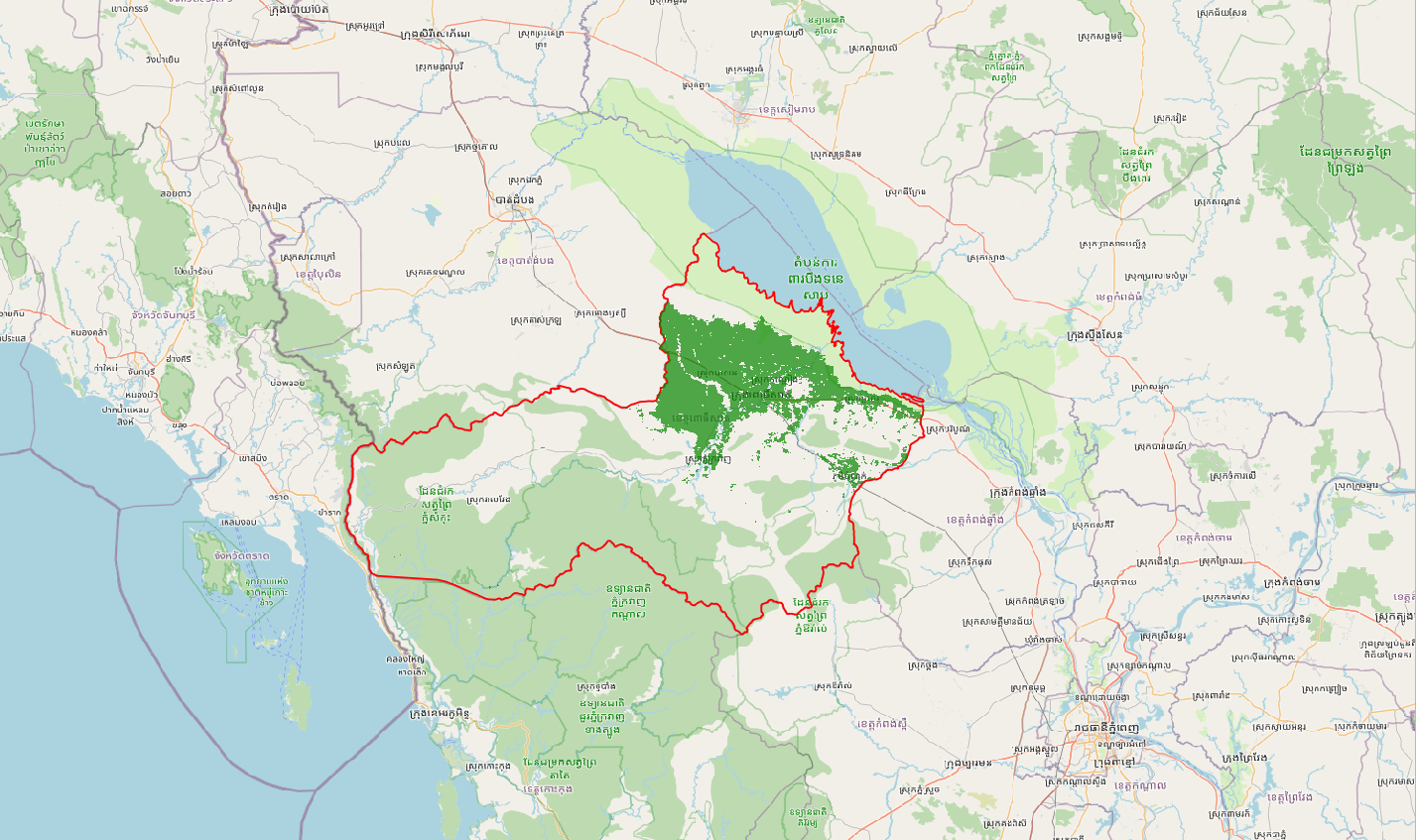
Visualize result of paddy area
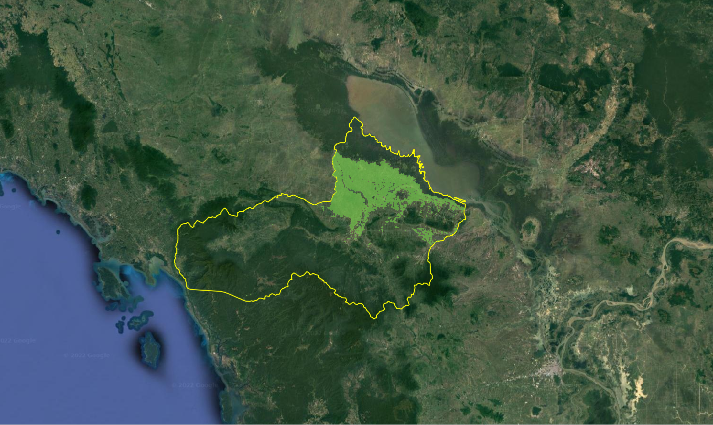
[26]:
from IPython.display import Image
Image(filename="images/paddy-area-result.png")
[26]:
[27]:
Image(filename="images/paddy-area-result-satellite.png")
[27]: